Autotune and Improving Flow Control Quality Through Response Time
Download this whitepaper as a PDF
Introduction
Flow control quality depends on many aspects of the system and its control elements. This article looks at flow control response time and the influences which may affect it. We look at how response time may be specified and measured, and we introduce manual and autotune methods to optimize the response for a given environment.
Flow Control Quality Depends on Response Time
Quality flow control is dependent on three aspects:
- a sensor that is accurate and repeatable
- a valve that can make small changes
- the speed of the control response (the speed at which sensor data can be read and the valve can be changed).
Many sensor technologies can provide acceptable accuracy and repeatability. Similarly, valves of a variety of designs can reliably impart large or small changes in flow. If the components are suitable for the application, then the flow control performance will be governed by the speed of the control response.
Accurate Setpoint Tracking
A device with a faster control response will more accurately track the setpoint as it changes. If the setpoint changes faster than the flow control device can respond, extra error will be introduced.
This is the primary reason why a flow control device with a faster response time will perform better than one with a slower response when embedded in a supervisory control loop (to control temperature, humidity, or other parameters crucial to the process).
Rejection of Disturbances and Errors
For very simple systems that are comprised of a good pressure regulator, a flow control device, and a simple process with little restriction, the flow control response speed will have little impact on the overall system performance. A good pressure regulator coupled with an orifice will maintain a desired flow rate for many applications. However, to maintain the flow over time in such a simple system, the pressures and temperatures in the system must remain constant. Any changes will be directly reflected in the flow rate.
Once dynamic elements are added into a system, such as valves that feed other devices in the process, disturbances can become the dominant factor in the performance of the system. The flow control response speed now becomes much more influential in providing quality flow control.
In Figure 1, a pressure wave moves through a system. This type of disturbance may occur with the closing of a valve upstream of this device that feeds another device. The four measurements were taken from the same flow controller optimized for different response times. The initial effect of the disturbance is the same for all control devices (the device does not choose the speed or size of the disturbances in the system). However, faster flow controller responses minimize the effects of the disturbance, keeping the flow closer to the desired setpoint and return to the setpoint faster.
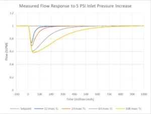
Figure 1. When a pressure wave is created by closing a valve to another device, a flow controller with a faster response time (blue) can mitigate the flow disturbance more quickly.
The example wave in Figure 1 is somewhat larger than would be expected in a well-designed system, and the exact effects of the disturbance depend on many factors, including details of the valve design. Nevertheless, this data is indicative of typical disturbances.
Optimized Response Speed vs Widely Varying System Conditions
A specific response is of limited use if it only works for some of the conditions that occur in the process. Because system characteristics can change significantly under different process conditions, achieving a reasonable response across all conditions may be preferable to having an excellent response in one condition and poor control in others.
Achieving broader, stable control is usually accomplished by checking and optimizing the flow controller response under multiple process conditions. The smallest control loop gains are then selected (sacrificing some response speed for stable control). Alternatively, the flow controller optimization may target a slower response speed than the device is nominally capable of for those specific conditions, which usually leads to more consistent performance (though also likely slower) across more conditions.
The most precise flow control will be achieved in a system that minimizes both the disturbances and the variety of conditions seen by the system and flow controller.
Flow Control Response Time Definition
Many manufacturers provide an indication of the expected flow control response time, but there are almost as many definitions of response time as there are vendors. For the purposes of this discussion, the response time is the sum of the dead time and the time constant of the first order response (Figure 2). For devices with integral valves, the dead time is usually small compared to the time constant and can typically be ignored.
Flow Control Response Time Details
The definition of response time (dead time plus time constant) is taken from time domain control system analysis and design. With this approach, the simplest useful model of a linear control system is called a First Order Plus Time Delay (FOPTD) model or a First Order Plus Dead Time (FOPDT) model. These models refer to the same concept with slightly different labels. As shown in Figure 2, following a command / setpoint change, some time elapses during which the dependent variable remains unchanged. This period is called time delay or dead time. After this delay, the response follows an exponential curve approaching a final value. The exponential time constant is the amount of time required to move 63.2% from the initial value to the new value.
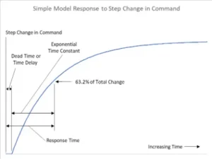
Figure 2. A simple but useful model of a step response in a control system.
Many control systems can be usefully approximated by this model. The model is less accurate, however, if the true system response deviates from a simple exponential form.
Alternative Flow Control Response Times
There are a number of alternative definitions of the flow control response time. Some of the more common ones are mentioned here for completeness:
- T63: This is the time required for the step response of the process to reach 63.2% of the total change. It sometimes includes the dead time and sometimes does not. For devices with integrated valves, the dead time is short enough that the two values are similar. The T63 value can be easily used in a first order control system model.
- T98: This is the time required for the step response to reach 98% of the total change. It sometimes includes the dead time and sometimes does not. It is often interpreted as the amount of time for the process to settle to within 2% of the final value, though this is not true for systems with significant overshoot. Also, to transform this value for use in a first order model of the controller requires the assumption that the control response closely follows an exponential form; this is often not the case.
- Rise Time: This is the time for the process to go between 10% of the total change and 90% of the total change. Rise Time is useful because it represents the bulk of the control response without being heavily influenced by the details of noise at the beginning of the change or any overshoot / undershoot that may occur. It cannot be transformed into a parameter for a first order model of the controller without assuming the form of the response.
- Settle Time / Settling Time: This is the time during which the process will be more than a given threshold value away from the final value. The threshold is usually stated as a percentage of the step size or a percentage of full scale. Sometimes this is taken to imply that there is no overshoot, but an optimization that modestly overshoots will often have a shorter settling time than one that has no overshoot. It cannot be transformed into a parameter for a first order model of the controller without assuming the form of the response.
- Bandwidth: This indicates how fast of a sine wave the controller can follow reasonably closely, typically given in hertz (Hz). While not a time, this is mentioned here because it is closely related to response time and is the most crucial parameter in frequency domain control analysis and design.
Influences on Flow Control Response Time
Flow Controller
As we mentioned earlier, quality flow control requires an accurate sensor, a sensitive valve, and optimized flow control response time.
Flow controller manufacturers generally provide expected response timings, but they may use different definitions to do so. Some vendors may specify the fastest response that the device can possibly achieve under ideal circumstances. Others cite times that are almost always reachable, though considerably better performance may be possible in many applications. With so much variation, it can be difficult to compare a flow control device’s actual capability without directly testing the device.
The fastest response a digital flow controller can reliably produce will be approximately the slowest of:
- The sensor response time constant
- The valve response time constant
- 10 sample intervals
These three values are often sufficient to form a general idea of the best possible performance when it is not possible to test the device first-hand. Some or all of this information may be available from the vendor, giving a sense of how aggressive or conservative a published control response time might be.
Sensor response
A control system cannot influence what it cannot sense; therefore, the control response cannot be faster than the response time of the sensor and the flow reading processing.
Valve response
Similarly, a controller cannot influence the flow faster than the valve can move. It is uncommon for the digital sample interval within a flow controller to be a limiting factor, though this is sometimes seen with communication lags between a flow controller and a supervisory controller.
Sampling intervals
If the sensor technology or sample interval is slow compared to the actual disturbances in the system (remember that the physical disturbances are not limited to the speed of the sensor), then non-repeatability or inconsistent process results may occur, with little or no indication from the flow controller about what is actually occurring in the system.
Rest of the System
The performance of simple systems will be limited almost purely by the flow controller performance. By adding just one restriction, however, the characteristics of the system might become the limiting factor. Most often, these characteristic times are driven by how pressure changes in the system. These pressure changes are commonly influenced by:
- The consistency of any pressure regulation in the system (typically upstream of the flow controller), and the timing of any variations in the regulated pressure
- The amount of restriction upstream or downstream of the controller, relative to the flow setpoint
- The volume downstream of the flow controller before any significant restrictions
For example, placing a large volume before a restriction (large compared to the amount of flow through the restriction) creates a system with a slower time constant that is usually more stable. If responsiveness is a priority, the volume and restrictions in the system downstream of the controller must be minimized. In either case, it is possible that the characteristic time of the system will change what can be done with the flow controller; optimizing the control loop for the exact system characteristics will yield the best performance for the combination of device and system.
Flow controllers that use a simple speed factor rather than configuring multiple closed loop control gains may not effectively incorporate system time constants differing from those used at the factory.
When to Optimize Flow Control Response Speed
It may make sense to optimize control in a variety of circumstances.
Initial Installation
A device will be configured at the factory to handle a broad range of typical conditions; however, those conditions will almost never exactly match the installation. Optimizing control in situ will maximize the flow control performance in that particular system.
Changes in the Process
Significant changes to how a system is used may change its characteristics. One common example is increasing or decreasing the system pressure, which may significantly change how the system responds. Optimizing the control can compensate for these changes.
The characteristics of the valve in a control device will determine exactly how flow control changes. Figures 3 and 4 show some typical variations.
In Figure 3, a flow controller has been optimized while the inlet pressure was 30 PSIG. When the inlet pressure is changed significantly, the control response is degraded, as evidenced in Figure 3 by the transients after a setpoint change. Optimizing the response time for the new process conditions can restore the level of performance.
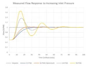
Figure 3. Increasing the system pressure after flow control has been optimized can decrease flow control stability. The instability here appears here as transients after a setpoint change. While these are more dramatic pressure changes than is common in a system, they illustrate the potential for how a change in system pressure can affect. Control can be optimized to achieve a very similar response for any pressure.
Figure 4 shows that the valve responds differently when the pressure is reduced slightly versus when the pressure is reduced even more. This kind of change in response depends on details of the valve design and is one of the reasons to optimize the response time for the physical process rather than relying on simple compensation models that may be built into a device but are unlikely to accurately reflect this kind of behavior.
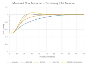
Figure 4. Decreasing the system pressure after flow control was optimized can slow down flow control, limiting the controller’s ability to track the setpoint and mitigate disturbances. While these are more dramatic pressure changes than typical, they illustrate the potential for changing flow control performance. Control can be optimized to achieve a very similar response for any pressure.
Another common process change is the gas flowing through the system. Even flow controllers that offer compensation for changes in gas properties can benefit from being optimized using the actual process gas.
Changes in the Physical System
Significant changes in system plumbing, such as the removal or addition of a volume or a restriction, are likely to impact flow control performance.
Figures 5 and 6 show a device that was optimized with a particular process volume downstream of the flow controller. Figure 5 shows how the response changes when the process volume was then increased, and Figure 6 shows the response with a decreased volume. Optimizing control can establish a similar response performance for either volume. These results are for an example system, the effects of changing volumes and restrictions can vary dramatically with the system setup and components used.
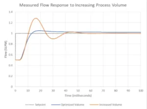
Figure 5. Increasing the process volume downstream of the flow controller, relative to the volume used when flow control was optimized can decrease flow control stability, which appears here as transients after a setpoint change. The effects of changing volumes or restrictions can vary widely; this is one sample system. Either setup can be optimized to achieve similar performance.
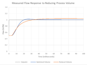
Figure 6. Decreasing the process volume downstream of the flow controller, relative to the volume used when flow control was optimized, can slow down flow control, limiting the controller’s ability to track the setpoint and mitigate disturbances. The effects of changing volumes or restrictions can vary widely; this is one sample system. Control can be optimized to achieve a very similar response for either volume.
Moving a Device Between Systems or Experiments
In some labs, a control device may be used in multiple experiments with very different configurations. Optimization will ensure performance whenever the device is moved to a new setup or when a setup is changed.
Improved Flow Control
In some situations, an exact response speed may be required to protect a sensitive process, or multiple devices may need to provide the same response within a connected system. Optimization can be used to reach a particular performance goal inside that system.
When flow control performance changes, the cause may not be readily apparent. Optimization can serve as a first step in troubleshooting, perhaps restoring the system to the desired performance. However, unexplained changes may indicate unexpected conditions in the system or flow controller and further investigation may be worthwhile.
Measuring Flow Control Response
The flow control response might be measured for a variety of reasons, but they usually fall into one of two categories: to characterize system performance and to diagnose / improve system performance. Common reasons to characterize system performance include using the flow controller in a supervisory control loop, or to see if the flow controller meets performance requirements as currently configured. Checking the response can also be a useful step when adjusting the system or flow controller configuration, or to see if the system has changed enough that control optimization may be worthwhile.
Manual Measurement
The flow control response can be completed manually by collecting data and calculating the relevant control parameters. Manual measurement, however, can be laborious and requires knowledge of control parameters and how to accurately calculate them. Some flow controllers may require analog equipment or extensive digital integration in order to collect the necessary data. Furthermore, establishing a sufficiently fast communication channel to gather that data may require a significant effort and may disrupt standard process communications.
Alicat LC/MC Check Control Function
Some controllers can conveniently capture and analyze their own control response without extra equipment or wiring. The controller always has access to all possible process data, even if available communications channels are limited. These results can then be provided in a simple to understand manner that requires minimal training to understand.
The Check Control feature in Alicat LC liquid flow controllers and MC model mass flow controllers with firmware 10v11 and later. (Figure 7) is an example of an in-device method that measures and reports widely used control metrics.
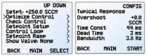
Figure 7. Automatically calculating system response variables with Check Control.
The Check Control function can be initiated from the device’s display, via text serial commands, or using industrial protocols such as Modbus RTU, EtherNet/IP, or PROFINET. During Check Control, the device completes a change to a user-provided setpoint, recording flow data for a user-specified time period. Following the change, several common control variables are reported:
Overshoot The amount of process overshoot observed as a result of the setpoint change.
Dead Time The amount of time between when the setpoint was changed and when the process began to change. This is also commonly called Time Delay and can be directly used as the delay parameter in a first order model of the controller.
Time Constant The amount of time required for the process to move 63.2% of the setpoint change after the process began to change. This can be directly used as the time constant parameter in a first order model of the controller.
Bandwidth The estimated frequency of the fastest sine wave setpoint that the device can reasonably follow; it is also expected to reject most sinusoidal disturbances with a lower frequency.
These parameters can be used to diagnose changes within the system, as well as to design or adjust a supervisory control system.
Optimizing Flow Control Response Speed
When the device settings are insufficient to provide good control in the current process conditions, the device response can be optimized, either manually or within the device.
Manual Optimization
There are many approaches to optimizing a control loop; many papers and entire books have been written on possible techniques and options. However, most will require additional equipment and knowledge of control system analysis and design.
Alicat LC/MC Optimize Control Function — Autotune
Alicat LC liquid flow controllers and MC model mass flow controllers (with firmware version 10v11 or later) can be autotuned—optimized automatically—from within the device. The functionality can be accessed from the device display, serial commands, or industrial protocols such as Modbus RTU, EtherNet/IP, or PROFINET.
a. 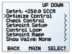 b.
b. 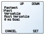 c.
c. 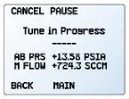 d.
d. 
Figure 8. Alicat Autotuning: a) selecting the function; b) choosing the Speed setting; c) optimization in progress; d) results following optimization.
During autotuning, the device moves to a series of setpoints. For each setpoint change, the device determines system properties and optimizes control parameters. When the parameterization is complete, the device response is adjusted to the optimal settings, and the device reports the overshoot, dead time, time constant, and bandwidth of a typical response with the final settings (described in the Check Control section above).
The autotune function is much faster than most manual techniques. For most devices, the process is completed in 30–90 seconds. Ultra-low flow devices (roughly 50 SCCM and below) may require longer; 0.5 SCCM devices may take up to 15 minutes.
Optimization is most effective when the process conditions maximize the pressure delta across the valve(s) involved. Unstable control may result when a device operates at a higher pressure delta or higher common mode pressure than it was optimized for. If operating conditions are expected to include higher pressures than are available for optimization, a speed level that emphasizes versatility is preferrable.
Optimization is more sensitive to fluctuations in the environment than normal closed loop control. Most fluctuations will result in control loop gains that are smaller than they might otherwise be, as it is difficult to separate the effects of the disturbance from the response of the system. Ultra-low flow and other slowly responding devices will be much more sensitive to disturbances or other fluctuations in the system.
Advanced Configuration
For most situations, Autotune will determine the best response time without any user input. The function can, however, be further configured to support atypical process requirements or specific control goals.
Speed
The Speed setting determines how the optimization will address the tradeoff between speed and the ability to handle more varied process conditions:
FAST is the default option which balances speed and versatility for most situations.
FASTEST maximizes response speed (i.e., minimize the control loop response time).
VERSATILE or MOST VERSATILE will provide a response speed that accommodates a wider range of conditions, but with the tradeoff of slower response. The system may not be able to respond to disturbances or quickly changing conditions.
Figure 9 shows the response of an example mass flow controller that has been autotuned using each Speed level. Figure 9 shows a typical variation across the speed levels though, as discussed above, the speed that is possible for a device in any particular system will vary.
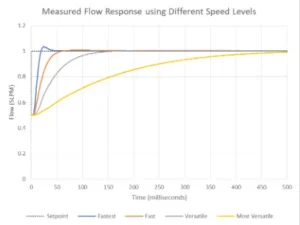
Figure 9. The impact of Speed settings on the speed of response.
In some instances, the process itself limits the response speed, and increasing the speed level may not make a difference. Optimization will still likely be a benefit, though the speed setting may not make a significant impact.
GOAL is a Speed option for advanced users who need to achieve a particular response profile or who need to configure multiple devices to provide the same response. The function will attempt to achieve the requested time constant. When the goal is impossible to meet (e.g., if the goal is set to 0), the nearest possible time constant will be used (which is equivalent to the FASTEST option).
Max Flow
During optimization, the device will move to a series of setpoints, some of which may be above the device’s current setpoint. The Max Flow setting limits the maximum flow during optimization for situations in which the process needs to be protected from excessive flows. In unusual circumstances the maximum flow may be exceeded; however, the device will attempt to minimize the duration. Giving the device a setpoint larger than the Max Flow used for control optimization may result in unstable control.
Loop Type
The optimization function will automatically use the best control algorithm based on the device, desired control speeds, and characteristics of the system. The AUTOMATIC option is, therefore, the default and recommended setting.
In some instances, advanced users may have specific requirements and may choose to specify either the PD2I or PDF closed loop algorithm during optimization.
Conclusion
Quality flow control requires a combination of careful system design and excellent flow control elements. The response of a control device will always be specific to the system and environment. Optimizing that response ensures that the device will provide the best flow control for any set of circumstances. In-device, autotuning greatly speeds up and simplifies the process, without requiring extensive knowledge of control systems and parameters.
Advantages of Autotune
- Fastest optimization process
- Fastest control system response time
- Tune control to the characteristics of the particular system
- Smoother flow over the range of process conditions
- Optimize system without additional equipment or control design expertise
- Run it by yourself